Yesterday I showed you how to use Column Validation to validate Social Security Numbers, Phone Numbers, Employee Numbers, Part Numbers, and other things with strict formatting. Today I’m going to expand on that idea by showing you something more complex—we’re going to validate that an acceptable email address has been entered.
The formula we’ll write in this post won’t catch every possible bad email address, but it’s designed to catch the most common mistakes. I’ll begin with the entire formula, then I’ll break it down and explain what’s going on piece by piece. This formula checks to see that the email address contains some characters, followed by an ampersand, more characters, a dot, and more characters—it also checks to make sure it doesn’t include a space character. Here is the formula:
=(LEN(LEFT([Email],FIND("@",[Email])-1))>0)
+(LEN(RIGHT([Email],LEN([Email])-FIND(".",[Email],FIND("@",[Email]))))>0)
+(LEN(MID([Email],FIND("@",[Email])+1,FIND(".",[Email],FIND("@",[Email]))-FIND("@",[Email])-1))>0)
+(ISERROR(FIND(" ",[Email]))=TRUE)
=4
Whew! What a formula. Let’s break it down…
Finding the Ampersand
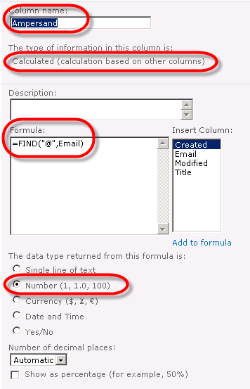
The first thing we want to do is find the position of the ampersand in the string the user enters. I’ve created a custom list to work with. I’ve added a column named Email (of type Single line of text) that will be where the user enters the e-mail address and I’ve added a calculated column named Ampersand to store the position of the ampersand (we won’t need this column for the validation, but it will help you understand how this formula works). We’ll use the FIND function to get this character location (Click here for details about all the formulas and functions that are available to you for column validation). The formula for the Ampersand column is =FIND(“@”,[Email]).
If we enter in an email address of test@testing.com, you’ll notice this column correctly populates with 5. 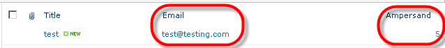
Find the Characters Before the Ampersand
You’ll remember that we need to make sure the ampersand isn’t the first character in the email address. So the next thing we want to do is get all the text that is before the email address. To do that we’ll add a calculated column named First and use the formula =LEFT([Email],FIND("@",[Email])).
This results in “test@”: 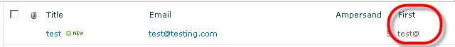
We don’t need the @ sign on the end of it, but the LEFT() function gives us everything up to and including the position we give it. So we’ll need to subtract one from it for it to be correct. Let’s change it to =LEFT([Email],FIND("@",[Email])-1). This gives us what we want. 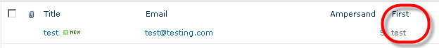
Now that we have that, we can see how many characters long it is by using the LEN() function. Let’s add another column named FirstLen that uses that function around all this, like so: =LEN(LEFT([Email],FIND("@",[Email])-1)).
You’ll notice this column contains 4 for the original example and it contains 0 if we enter in an email address of just “@.” 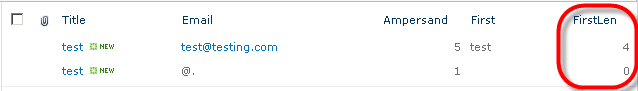
We know that this length must be greater than zero to validate, so, with that we now we have the first part of our column validation for the Email column:
=(LEN(LEFT([Email],FIND("@",[Email])-1))>0)
If we enter this and try to add an email address that begins with an ampersand, or doesn’t contain an ampersand at all, we’ll get an error. 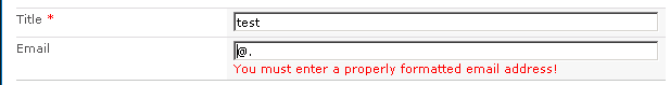
Find the Characters After the Dot
You’ve probably already figured out that you can find the location of the dot by using the formula =FIND(".",[Email]). However, if someone enters an email address with a dot before the ampersand (such as testy.tester@testing.com) this will cause a problem for our formula. We need to find a dot that is after the ampersand. We can modify the FIND() formula to start looking where the ampersand is though by changing it to: =FIND(".",[Email],FIND("@",[Email])).
Let’s create a calculated column called dot with this formula. Notice this correctly shows us the position of a dot that is after the ampersand. 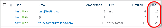
We’re almost ready to use the RIGHT() function to extract the characters we need. Let’s create a calculated column named Right and use the formula: =RIGHT([Email],FIND(".",[Email],FIND("@",[Email])))
You’ll notice this gives us far more than just the few characters we want: 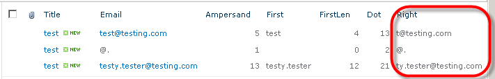
This is because the RIGHT() function begins with the character we give it from the left, not from the right. So we need to translate that to characters from the right. We can do that by simply subtracting that number from the length of the whole string using the LEN() function. Let’s modify the formula like this: =RIGHT([Email],LEN([Email])-FIND(".",[Email],FIND("@",[Email]))
This gives us what we want. 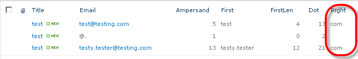
Now we just need to get the length of that piece. We’ll create a new calculated column called RightLen and use the formula: =LEN(RIGHT([Email],LEN([Email])-FIND(".",[Email],FIND("@",[Email]))))
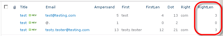
Since this is working correctly, we can add that to our validation rule on the Email column to check to make sure this value is greater than zero. Here is the Email Validation formula so far:
=(LEN(LEFT([Email],FIND("@",[Email])-1))>0)
+(LEN(RIGHT([Email],LEN([Email])-FIND(".",[Email],FIND("@",[Email]))))>0)
=2
If we try to enter an email address without a top level domain on the end, we get the error. 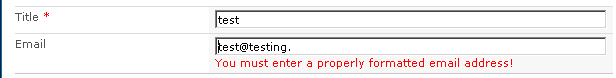
Find the Characters Between the Ampersand and the Dot
We can’t have a valid email address without a domain name between the ampersand and the dot. So now we need to figure out how to check for that. For this we’ll use the MID() function and all the skills you’ve learned up to this point. Create a new calculated column named Middle and use the formula: =MID([Email],FIND("@",[Email])+1,FIND(".",[Email],FIND("@",[Email]))-FIND("@",[Email])-1)
This correctly gives us the domain name of the email address: 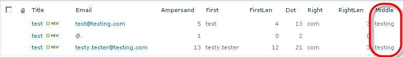
We’ll create a calculated column named MiddleLen and wrap the formula in a LEN() function to give the length of this part, like so: =LEN(MID([Email],FIND("@",[Email])+1,FIND(".",[Email],FIND("@",[Email]))-FIND("@",[Email])-1))
This correctly gives us: 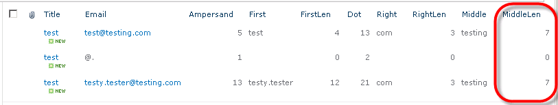
We now have the bulk of our email validation formula done. We just need it to check if the length of all three parts is greater than zero. Here is the Email Validation formula so far:
=(LEN(LEFT([Email],FIND("@",[Email])-1))>0)
+(LEN(RIGHT([Email],LEN([Email])-FIND(".",[Email],FIND("@",[Email]))))>0)
+(LEN(MID([Email],FIND("@",[Email])+1,FIND(".",[Email],FIND("@",[Email]))-FIND("@",[Email])-1))>0)
=3
If we try to use this and leave out the domain portion, we’ll get an error. 
Check for Spaces in the Email Address
As a final addition to our formula, we’re going to check for a space in the email address. We know that it’s easy to accidentally press the space-bar while typing, but spaces aren’t allowed.
Let’s add a new calculated column named SpacePos and use the following formula to find the position of any space: =FIND(" ",[Email])
Notice the column contains a #VALUE error if the Email address doesn’t contain a space and the position of the space character if it does. 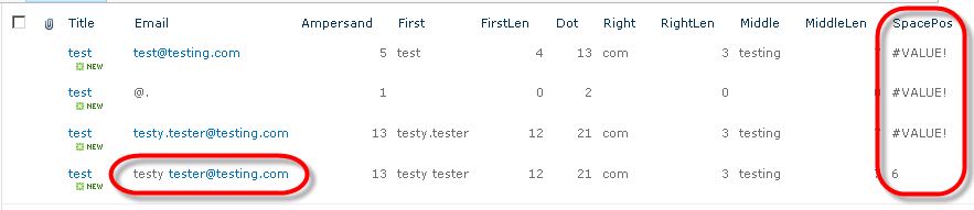
There is another function called ISERROR() that allows us to check for these kinds of errors. Change the formula on the SpacePos column to: ISERROR(FIND(" ",[Email]))
Notice that the ones that don’t contain a space evaluate to TRUE and the one that does evaluates to FALSE: 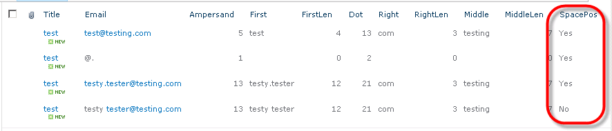
We can now use this as a fourth piece of criteria to check in our formula by adding it to our email validation formula. Here is the complete formula:
=(LEN(LEFT([Email],FIND("@",[Email])-1))>0)
+(LEN(RIGHT([Email],LEN([Email])-FIND(".",[Email],FIND("@",[Email]))))>0)
+(LEN(MID([Email],FIND("@",[Email])+1,FIND(".",[Email],FIND("@",[Email]))-FIND("@",[Email])-1))>0)
+(ISERROR(FIND(" ",[Email]))=TRUE)
=4
More…
I hope this has been helpful and inspires you to do more serious data validation. If it does, please share any helpful formulas you discover in the comments. If you have things that you just can’t seem to figure out how to validate, share those as well and perhaps someone else can help with those. Almost anything you need to validate is possible with a little work.